# Define operation periods for treatments::::::::::::::::::::::::::::::::::::::::::
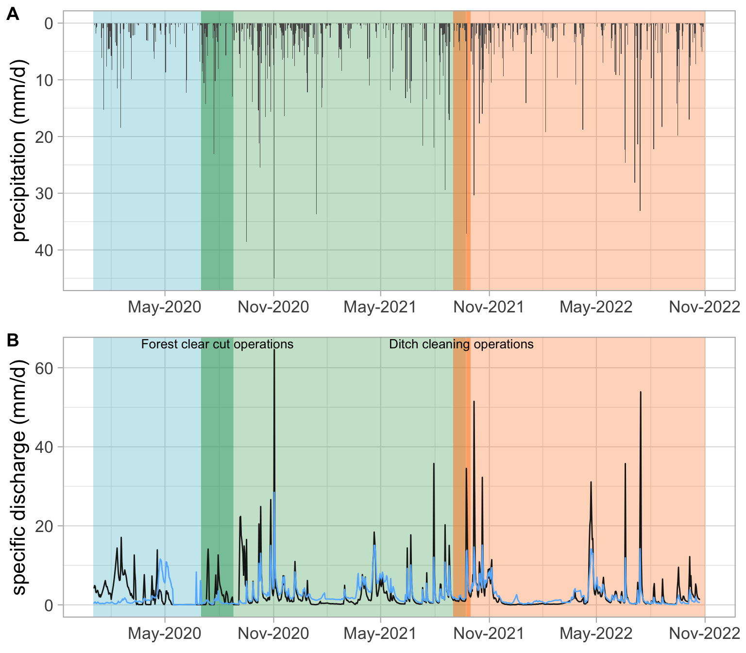
predisturbance_start = as.Date("2020-01-01")
predisturbance_end = as.Date("2020-07-13")
clearcut_start = as.Date("2020-07-01")
clearcut_end <- as.Date("2020-08-25")
postharvest_start = as.Date("2020-07-14")
postharvest_end= as.Date("2021-09-13")
ditch_cleaning_start <- as.Date("2021-09-01")
ditch_cleaning_end <- as.Date("2021-09-30")
postditch_start = as.Date("2021-09-14")
postditch_end= as.Date("2022-11-01")
# Timeseries 14C per site, CO2 and DOC seperately
plot_timeseries = function(data, y_var,labs_y,
ymin_rect, ymax_rect)
{
ggplot(data, aes(x=Date, y=!!sym(y_var),
group=Site_id, color=Site_id,
fill=Site_id, shape=Site_id)) +
# Add gray background bars for operations
annotate("rect", xmin = predisturbance_start, xmax = predisturbance_end,
ymin = ymin_rect, ymax = ymax_rect,
fill = "#3CB7CC", alpha = 0.3) +
annotate("rect", xmin = postharvest_start, xmax = postharvest_end,
ymin = ymin_rect, ymax = ymax_rect,
fill = "#32A251", alpha = 0.3) +
annotate("rect", xmin = postditch_start, xmax = postditch_end,
ymin = ymin_rect, ymax = ymax_rect,
fill = "#FF7F0F", alpha = 0.3) +
annotate("rect",
xmin = clearcut_start, xmax = clearcut_end,
ymin = ymin_rect, ymax = ymax_rect,
fill = "#32A251",, alpha = 0.5) +
annotate("rect",
xmin = ditch_cleaning_start, xmax = ditch_cleaning_end,
ymin = ymin_rect, ymax = ymax_rect,
fill = "#FF7F0F", alpha = 0.5) +
geom_line(data=data[!is.na(data[[y_var]]), ]) +
geom_point(size=3, aes(color = Treatment)) +
scale_x_date(limits=c(as.Date("2020-01-01"), as.Date("2022-11-01")),
date_labels = "%b-%Y", date_breaks = "6 months") +
scale_color_manual(values=c(site_colors))+
scale_fill_manual(values=alpha(c(site_colors), 0.7))+
scale_shape_manual(values=c(site_symbols))+
labs(y=labs_y)+
theme( # set margins to align combined plots
plot.margin = margin(5.5, 5.5, 5.5, 5.5, "pt"),
axis.text.x = element_text(size = 10),
axis.title.x = element_text(size = 11),
panel.grid.major = element_line(size = 0.5),
panel.grid.minor = element_line(size = 0.25)
)
}
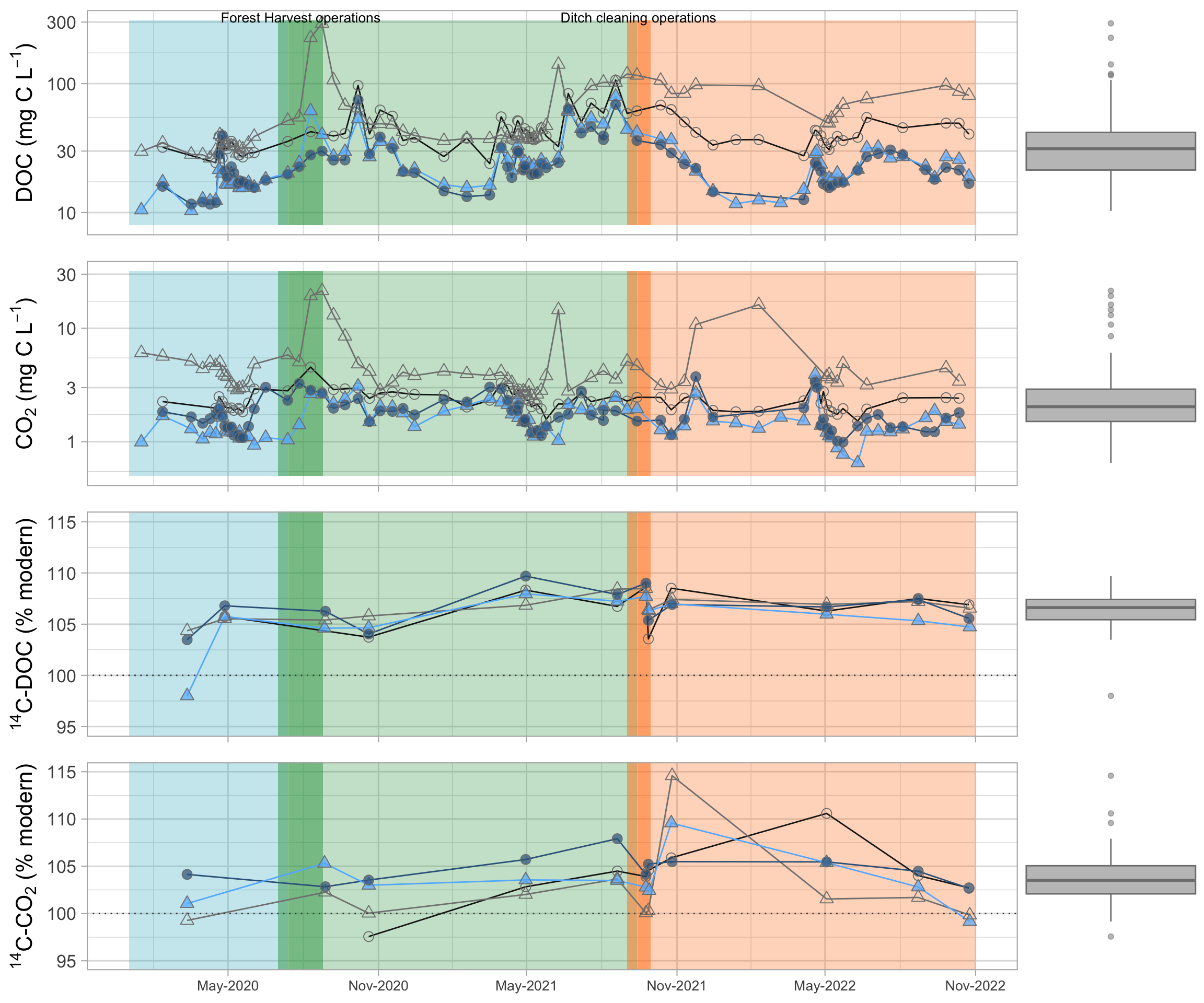
#Concentration timeseries
timeserie_DOC = ggExtra::ggMarginal(
plot_timeseries(DC_Q, #%>% filter(Site_pairs == "FC")
"DOC_mgL", "DOC (mg/L)",
ymin_rect=8, ymax_rect=310
)+
# Add text labels for operations
annotate("text", x = clearcut_start + (clearcut_end - clearcut_start)/2, y = Inf,
label = "Forest Harvest operations",
vjust = 1.2, hjust = 0.5, size = 3.5, color = "black") +
annotate("text", x = ditch_cleaning_start + (ditch_cleaning_end - ditch_cleaning_start)/2, y = Inf,
label = "Ditch cleaning operations",
vjust = 1.2, hjust = 0.5, size = 3.5, color = "black") +
labs(y=bquote("DOC (mg C L"^-1*")"))+
scale_y_log10()+
#facet_wrap(~Site_pairs)+
theme(legend.position = "none", axis.title.x = element_blank(), axis.text.x = element_blank()),
margins=c("y"), type = "boxplot", groupColour = TRUE, groupFill = TRUE )
timeserie_CO2 = ggExtra::ggMarginal(
plot_timeseries(DC_Q, #%>% filter(Site_pairs == "FC"),
"CO2_mgL", "CO2 (mg/L)",
ymin_rect=0.5, ymax_rect=32)+
labs(y=bquote("CO"[2]*"\n (mg C L"^-1*")"))+
scale_y_log10()+
# facet_wrap(~Site_pairs)+
geom_abline(y=100)+
theme(legend.position = "none", axis.title.x = element_blank(),axis.text.x = element_blank()),
margins=c("y"), type = "boxplot", groupColour = TRUE, groupFill = TRUE )
timeserie_14CDOC = ggExtra::ggMarginal(
plot_timeseries(DC_Q, #%>% filter(Site_pairs == "FC"),
"DOC_14C_Modern", "14C-DOC (%)",
ymin_rect=-Inf, ymax_rect=Inf)+
scale_y_continuous(limits=c(95,115))+
#facet_wrap(~Site_pairs)+
labs(y = expression(""^14*"C-DOC (% modern)"))+
geom_hline(yintercept =100, linetype="dotted", color="grey30")+
theme(legend.position = "none", axis.title.x = element_blank(),
axis.text.x = element_blank()),
margins=c("y"), type = "boxplot", groupColour = TRUE, groupFill = TRUE )
timeserie_14CCO2 = ggExtra::ggMarginal(
plot_timeseries(DC_Q,# %>% filter(Site_pairs == "FC"),
"CO2_14C_Modern", "14C-CO2 (%)",
ymin_rect=-Inf, ymax_rect=Inf)+
scale_y_continuous(limits=c(95,115))+
#facet_wrap(~Site_pairs)+
geom_hline(yintercept =100, linetype="dotted", color="grey30")+
labs(y = expression(""^14*"C-CO"[2]*" (% modern)"))+
theme(legend.position = "none", axis.title.x = element_blank()),
margins=c("y"), type = "boxplot", groupColour = TRUE, groupFill = TRUE )
# Combine four plots
combined_timeseries= ggarrange( timeserie_DOC,
timeserie_CO2,
timeserie_14CDOC,
timeserie_14CCO2,
ncol = 1, align='v'#,
#heights = c( 0.45, 0.55, 0.45, 0.55) #, #labels="AUTO"
)
combined_timeseries